Table of contents:
Course material
The course uses the book Algorithm designs by Kleinberg and Tardos, ISBN: 9781292023946
Chapters and goals
Below follows an overview of each chapter in the book as well as the most central goals
Chapter 1 - Introduction: Some Representative Problems
We start with an introduction of several representative problems, which introduce you to the world of algorithms.
Goals 🏁
The student should be able to:
- Understand the Stable Matching Problem
- Understand how the Gale-Shapley algorithm solves the stable matching problem
- Understand some representative problems
Chapter 2 - Basics of Algorithm Analysis
Analyzing algorithms involves thinking about how their resource requirements—the amount of time and space they use—will scale with increasing input size.
Goals 🏁
The student should be able to:
- Understand the different definitions of an efficient algorithm
- Understand asymptotic notation and the asymptotic bounds \(O\), \(\Omega\), \(\Theta\) as well as their properties
- Understand how the stable matching problem is implemented using arrays and lists
- Have knowledge of common running-time bounds and some of the typical approaches that lead to them
- Understand what a priority queue is and how heaps are used to implement them
Chapter 3 - Graphs
One of the most fundamental and expressive data structures in discrete mathematics
Goals 🏁
The student should be able to:
- Understand the basic definition of a graph
- The difference between a graph and a directed graph
- Know of examples of applications of graphs
- Understand what a tree is and their properties
- Understand BFS - Breadth-First Search
- Understand DFS - Depth-First Search
- Understand how graphs are implemented
- Understand Directed Acyclic Graphs and Topological Ordering
Chapter 4 - Divide and Conquer
Divide and conquer refers to a class of algorithmic techniques in which one breaks the input into several parts, solves the problem in each part recursively, and then combines the solutions to these subproblems into an overall solution. In many cases, it can be a simple and powerful method.
Goals 🏁
The student should be able to:
- Understand the divide and conquer algorithm design method
- Understand mergesort
- Understand how its ideas are used to solve the Counting Inversions problem
- Understand the Finding the Closest Pair of Points problem
- Understand the Integer Multiplication problem
- Solve a recurrence by “unrolling” it
- Solve a recurrence by using substitution
Chapter 5 - Greedy Algorithms
An algorithm is greedy if it builds up a solution in small steps, choosing a decision at each step myopically to optimize some underlying criterion. One can often design many different greedy algorithms for the same problem, each one locally, incrementally optimizing some different measure on its way to a solution
Goals 🏁
The student should be able to:
- Understand the different Interval Scheduling problems
- Understand the Optimal Caching Problem
- Understand the Shortest Path Problem and how Dijkstra’s algorithm solves it
- Know what a Minimum Spanning Tree is and understand the Minimum Spanning Tree Problem
- Understand Prim’s and Kruskal’s algorithm
- Understand Huffman and Huffman Codes
Chapter 6 - Dynamic Programming
The basic idea of Dynamic Programming is drawn from the intuition behind divide and conquer and is essentially the opposite of the greedy strategy: one implicitly explores the space of all possible solutions, by carefully decomposing things into a series of subproblems, and then building up correct solutions to larger and larger subproblems.
Goals 🏁
The student should be able to:
- Understand the Dynamic Programming design method
- Understand when and how dynamic programming could be used
- Understand how dynamic programming tables are used
- Understand The Knapsack Problem
- Understand how dynamic programming can be used to solve the Longest Common Subsequence problem
- Understand how dynamic programming can be used to find Sequence Alignment
- Understand how dynamic programming can be used to find the Shortest path in a graph
- Find the asymptotic running time for Dynamic Programming Algorithms.
Chapter 7 - Network Flow
In graph theory, a flow network is a directed graph where each edge has a capacity and each edge receives a flow. The amount of flow on an edge cannot exceed the capacity of the edge. While the initial motivation for network flow problems comes from the issue of traffic in a network, we will see that they have applications in a surprisingly diverse set of areas and lead to efficient algorithms not just for Bipartite Matching, but for a host of other problems as well.
Goals 🏁
The student should be able to:
- Understand the Maximum-Flow Problem
- Understand the Ford-Fulkerson Algorithm
- Understand and solve the problem of Minimum Cut in a graph.
- Use Network Flow to solve The Bipartite Matching Problem
- Identify problems that can be solved using network flow.
Chapter 8 - NP and Computational Intractability
So far we’ve developed efficient algorithms for a wide range of problems and have even made some progress on informally categorizing the problems that admit efficient solutions. But although we’ve often paused to take note of other problems that we don’t see how to solve, we haven’t yet made any attempt to actually quantify or characterize the range of problems that can’t be solved efficiently.
Goals 🏁
The student should be able to:
- Understand the difference between P, NP, NP-Complete and NP-Hard problems.
- Prove whether a problem is NP or NP-Complete.
- Understand the basis of Polynomial-Time Reduction
- Understand the Satisfiability Problems
- Understand the Traveling Salesman Problem
- Understand the Hamiltonian Cycle Problem
Asymptotic notation
Asymptotic notation is an important tool when analyzing the runtime of an algorithm, they are used to set upper and lover bounds to how fast our algorithm runs. We calculate the running time by counting how many iterations the algorithm will run with an input of \(n\).
We use three different notations:
- Upper bound \(O\) (big-O) -> \(O(n)\) means that the function grows at a rate of at most \(n\)
- Lower bound \(\Omega\) (Omega) -> \(\Omega(n)\) means that the grows at a rate of at least \(n\)
- Asymptotically tight bound \(\Theta\) (Theta) -> \(\Theta(n)\) means that the grows at a rate in the exact order of \(n\)
When writing in asymptotic notation we always simplify to the asymptotically strongest variable. We remove all contants.
Meaning a function like \(3n^2 + 2n + 2 = \Theta(n^2)\)
What do we mean when we say asymptotically strongest?
Well we rank the runtimes of our algorithms based on how fast they grow asymptotically, here are some common runtimes sorted from fastest to slowest:
\[\Theta(1)\] \[\Theta(\log n)\] \[\Theta(n)\] \[\Theta(n^2)\] \[\Theta(2^n)\] \[\Theta(n!)\] \[\Theta(n^n)\]Analyzing an algorithms complexity
The complexity of an algorithm is the number of steps it takes to run it. Lets look at this simple algorithm that finds the largest number in an array, some lines are marked with numbers that are explained below.
def find_largest(arr: list):
    n = len(arr) # (1)
    largest = arr[0] # (2)
    for i in range(n): # (3)
        if arr[i] > largest:
            largest = arr[i]
    return largest
(1) n is the size of the input (in this case the length of the array of numbers, but n can also be number of users on a website, size of an image or the number of nodes in a graph (more on that later).
(2) This line runs only once, no matter the size of \(n\), this is often refferred to as a constant time operation. And is usually ignore when analyzing an algorithm.
(3) Here we loop over all the elements in the array, from \(0\) to \(n\). Every line inside this loop is then executed \(n\) times.
In total this algorithm will have a time complexity of (adding up how many times each individual line is run)
\[1 + 1 + n + n + n + 1 =3+3n=\Theta(n)\]Usually though, we can skip this initial exact calculation by only looking at the number of loops, and especially nested loops and recursively calling functions. In the following snippet that looks for duplicate numbers in an array, we can quickly see that there is two loops inside eachother that both run \(n\) times, so all lines inside the deepest loop will run \(n * n\) times, and the complexity is then \(\Theta(n^2)\)
def find_duplicate(arr: list):
    n = len(arr)
    duplicate_exists = False
    for i in range(n):
        for j in range(n):
            if i == j:
                # don't compare an element to itself (skip)
                continue
            if arr[i] == arr[j]:
                duplicate_exists = True
    return duplicate_exists
For functions that can return (stop) at different points we have to evaluate both the best and worst case scenario. Lets tweak the above snippet a little.
def find_duplicate(arr: list):
    n = len(arr)
    for i in range(n):
        for j in range(n):
            if i == j:
                # don't compare an element to itself (skip)
                continue
            if arr[i] == arr[j]:
                return True
    return False
For this snippet the worst case (\(O\)) is still the same \(O(n^2)\), but this only happens if there are no duplicates in the array. If there are duplicates the algorithm will return at the first duplicate it finds, in the best case (\(\Omega\)) the first two elements are duplicates. This means we also have a best case of \(\Omega(1)\).
We can never know for sure which case will happen, so we have to specify both the best and worst case scenario. See for instance The time complexity table of normal sorting algorithms as an example and see if you tell what is a good, or bad, sorting algorithm simply by their time complexities.
Data structures
When creating and evaluating algorithms to solve various problems, a good starting point is figuring out how the problem can be represented/stored in a data structure. These data structures are not directly covered in the book so we will give you a brief explanation and visualization of the most common ones here.
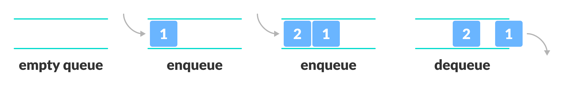
Queue
A queue is something we are all familiar with from waiting in line. It is a data structure that is used to store data in a first-in-first-out (FIFO) manner. The first element added (enqueued) to the queue is the first element to be removed (dequeued).
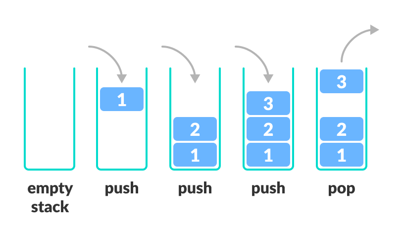
Stack
A stack is a data structure that is used to store data in a last-in-first-out (LIFO) manner. The last element added to the stack is the first element to be removed. Think of a stack of papers, when adding (pushing) to the stack you put the piece of paper on top, and when removing (popping) a piece of paper you take the paper back off the top again.
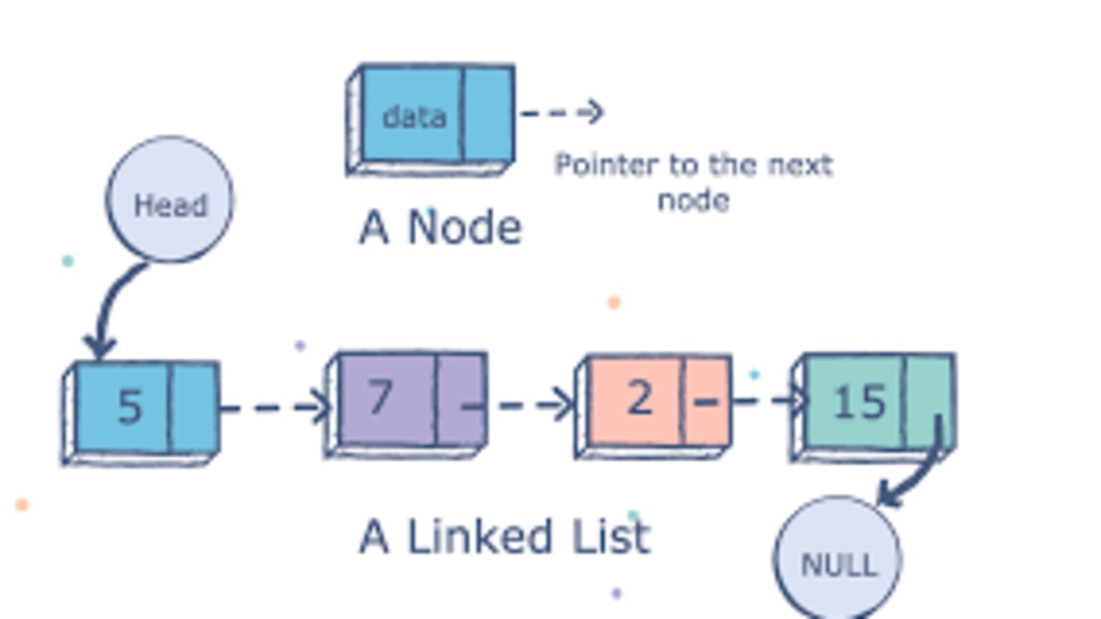
Linked List
A linked list is a linear data structure that consists of a sequence of nodes, each of which contains a piece of data and a reference to the next node in the sequence. The first node in the sequence is called the head node, and the last node is called the tail node. the tail nodes reference points to nothing or NULL. To traverse the list one can then start at the head node and follow the references to the next node until the tail node is reached. When adding a new node, it is simply added as a new tail node, making the previous tail node reference the new one.
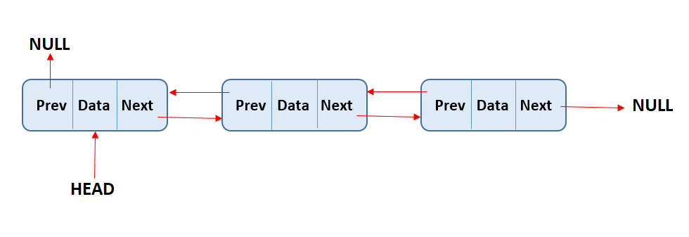
Linked lists can be implemented in only one direction (called Singly Linked List) shown above, or in both directions(called a doubly linked list). These linked lists contain an additional link to the previous node, which makes inserting/deleting nodes in the middle of the list easier. This is also one of the benefits of using linked lists instead of regular lists or arrays. Let’s say you have an array of length 10 000, if you wanted to insert a new element at index 0 you would have to shift every element in the array one position to the right before index 0 is freed. Using a linked list we instead just need to change the head of the linked list to the new node and link the previous head to the new head.
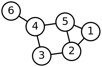
Graph
From math, you are probably used to talking about graphs in relation to functions in the form of \(f(x)=y\). However, in regards to computer science, a Graph is simply a collection of nodes and edges which form a network. This network is referred to as a graph.
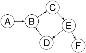
Graphs can also be directional, in the same manner, that a linked list can only contain references in a single direction. These are called directed graphs.
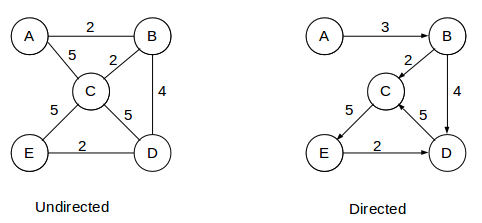
In addition to this, the edges of a graph can be weighted. this weight can represent anything, be the distance to travel between two nodes, the time between them, ticket costs, etc.
Tree
A tree is a graph structure that contains one node as the root. This root then has an arbitrary number of children, which are also nodes. The children of the root are called the branches. Nodes that do not contain any children are called leaves. The difference between trees and other graphs (besides the fact that it has a root) is that there are no cycles or circular referencing. When discussing the efficiency of trees we might talk about the tree’s height, which is the number of levels in the tree, or in other words, the largest number of edges from the root to the most distant leaf node. (the tree depicted below has a height of 3).
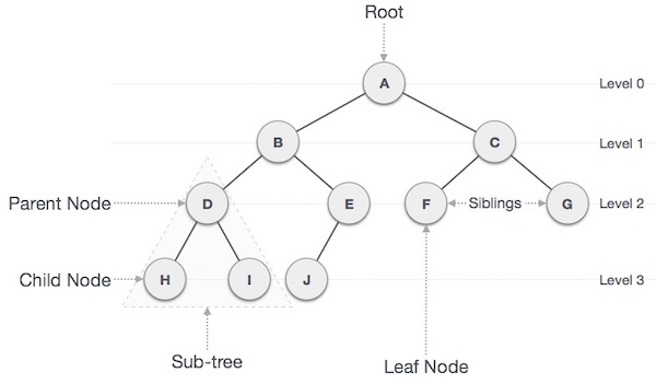
A notable version of trees are binary trees. A binary tree is a tree that has a maximum of 2 branches, or children, from each node. These types of trees can be particularly useful for searching algorithms, as an example below you can see how from the root you can easily check if a number exists in the tree by going right if the number is higher than the node, and left it the number is lower. Check yourself by checking if the tree contains the number 4 by searching from the root.
